I realize that most people have never learned about linear dynamical systems. It’s a pity, because it’s a very beautiful and useful area of applied math. In the next few posts I’m going to give a crash course on linear dynamical systems, which I hope will convey some sense of why they’re important. For more information check out my advisor’s class. I’ll start here with the most fundamental of the fundamentals.

State vector

The first concept in linear dynamical systems is the state vector. The state vector encapsulates all the relevant information about the system. For example, the state vector of a cannonball might contain its position and velocity. Suppose that the cannonball at time \(t\) has traveled 10 meters, has a height of 4 meters, and a velocity of 3 m/s forward and 1 m/s up. Then we might write the state vector as

Here \(x_t\) is a 4-dimensional vector (formally, \(x_t \in \mathcal{R}^4\)). The first entry is the forward distance. The second entry is the height. The third entry is the velocity forward. The fourth entry is the velocity up. For convenience, we will sometimes use the format \(x_t = (10,4,3,1)\) instead of the bracket notation above.

The dynamical system yields a series of state vectors \(x_0,x_1,x_2,\ldots\) for as long as we keep track! Generally we’ll use \(x_0\) to denote the initial, starting state and \(x_T\) to denote the terminal, ending state.

Dynamics matrix

The second important concept is the dynamics matrix. In our cannonball example, the dynamics matrix would be a \(4 \times 4\) matrix \(A\) (\(A \in \mathcal{R}^{4 \times 4}\)), such that

In words, given the state at time \(t\), we get the state at time \(t+1\) by multiplying the state at time \(t\) by the dynamics matrix.

Let’s make things concrete. We’re going to ignore gravity and assume our cannonball is flying through space, and that the timestep is 1 second (i.e., the interval between \(t\) and \(t+1\)). Our dynamics matrix will be

Let’s see how this works out, by multiplying our state vector \(x_t = (10,4,3,1)\) by \(A\). We get

In one second, the cannonball moves forward 3 m, for 13 m of forward distance total, and up 1 m, for a total height of 5 m. The velocities don’t change.

We’ll finish up this section by incorporating gravity. Each second the velocity up goes down by 9.8 m/s. We change our update rule to

Is this still a linear dynamical system? Yes, we just need to expand the state vector and the dynamics matrix! Instead of \(x_t = (10,4,3,1)\), we add the acceleration as a fifth entry and get \(x_t = (10,4,3,1,-9.8)\). And we change \(A\) to track the acceleration and apply it to the upward velocity:

Let’s do the math one more time:

See how that works?

Numerical example

For fun, here’s code for our cannonball example.

import numpy as np
import matplotlib.pyplot as plt
%matplotlib inline

# The state vector x_t.
xt = np.array([10,4,3,1])
print("The state vector x_t =", xt)
# The dynamics matrix A.
A = np.array([[1, 0, 1, 0],
              [0, 1, 0, 1],
              [0, 0, 1, 0],
              [0, 0, 0, 1]])
print("The dynamics matrix A:")
print(A)
print("The state vector x_{t+1} =", A@xt)

# Adding gravity.
A = np.array([[1, 0, 1, 0, 0],
              [0, 1, 0, 1, 0],
              [0, 0, 1, 0, 0],
              [0, 0, 0, 1, 1],
              [0, 0, 0, 0, 1]])

# Let's go for a ride!
T = 6 # Number of time steps.
# Initial state.
x0 = np.array([0,0,5,20,-9.8])
# Matrix to store all the state vectors.
X = np.zeros((5, T))
X[:,0] = x0
# Compute all the state vectors.
for t in range(T-1):
    X[:,t+1] = A@X[:,t]
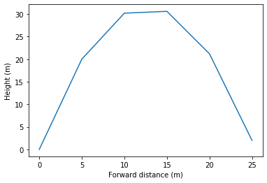
# Plot distance forward (x) vs height (y).
x = X[0,:]
y = X[1,:]
plt.plot(x, y)
plt.xlabel("Forward distance (m)")
plt.ylabel("Height (m)")
plt.show()

The state vector x_t = [10  4  3  1]
The dynamics matrix A:
[[1 0 1 0]
 [0 1 0 1]
 [0 0 1 0]
 [0 0 0 1]]
The state vector x_{t+1} = [13  5  3  1]