
Linear dynamical systems in unexpected places
In my PhD, I studied convex optimization, which is a sub-field of numerical optimization. The essence of convex optimization is restricting what’s allowed in an optimization model, in return for getting an optimization problem that can be solved quickly and reliably, with generic frameworks like CVXPY.
It may seem unnecessarily limiting to insist that an optimization problem be convex. Non-convex optimization is used with great success in many fields, including deep learning. Moreover, it takes a lot of expertise to model a problem in a convex way. If you create a mathematical model without experience in convex optimization, you will almost certainly end up with something non-convex. Creating convex models is a difficult skill!
I’ve thought a lot about why convex optimization is still worth talking about. My best argument is that there are still many places out there where convex optimization can be applied, and finding those places will unlock new scientific possibilities. I’ve spent the last two years looking for such applications, and I’ve found some interesting candidates.
The most promising candidate in my mind is log-linear dynamical systems (LLDS). LLDS are a model for how positive quantities change over time. In the linked paper we apply LLDS to hare and lynx populations. The advantage of modeling populations with LLDS, rather than a traditional predator-prey model, is that (1) we can trivially scale up the model to thousands of species and (2) we can control the population trajectory using convex optimization.
I believe LLDS can also be used to model chemical concentrations during chemical reactions (remember, positive quantities). I make a mathematical argument in the linked paper, but I could not find an easy way to test the theory empirically. I have very little experience with chemistry or chemical engineering, so I don’t even know where to start. (Side note, I know about flux balance analysis. The LLDS model, if applicable, is much more powerful.)
Numerical experiment
I found a Youtube tutorial on “Chemical Reaction Differential Equations in Python”, which shows how to simulate chemical reactions. Below I replicate the tutorial, and after each simulation show that the process can be modeled by a linear dynamical system. I would appreciate any feedback on the experiment or suggestions for future directions! (Contact info)
# Imports.
from scipy.integrate import odeint
import numpy as np
import matplotlib.pyplot as plt
import cvxpy as cp
%matplotlib inline
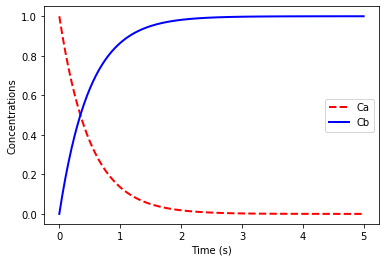
We first consider the reaction A -> B, with \(A_0 = 1.0\), \(B_0 = 0\) and reaction rates given by
\[\frac{dC_A}{dt} = -kC_A, \qquad \frac{dC_B}{dt} = kC_A\]where \(k=2.0\).
# Simulating the reaction.
def rxn(C,t):
    Ca = C[0]
    Cb = C[1]

    k = 2.0
    dAdt = -k * Ca
    dBdt = k * Ca

    # Return the derivatives.
    return [dAdt, dBdt]

t = np.linspace(0, 5, 100)
C0 = [1,0]
# Integrate the ODE to get the concentrations
# Ca and Cb at each time t.
C = odeint(rxn, C0, t)
# Plot the concentrations.
plt.plot(t, C[:,0],'r--',linewidth=2.0)
plt.plot(t, C[:,1],'b-',linewidth=2.0)
plt.xlabel('Time (s)')
plt.ylabel('Concentrations')
plt.legend(['Ca','Cb'])
plt.show()
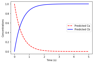
# Fitting a linear dynamical system to the time series data.
X = C.T
# Define a CVXPY variable for the dynamics matrix A.
A = cp.Variable((2,2))
# We predict the concentrations at time t+1 by multiplying
# the vector of concentrations at time t by the matrix A.
Xpred = A@X
# We find the A that minimizes the squared error
# of the prediction.
loss = cp.sum_squares(Xpred[:,:-1] - X[:,1:])
prob = cp.Problem(cp.Minimize(loss))
result = prob.solve()
print("The error in the linear dynamical system fit is", result)
print("The A matrix:")
print(A.value)

# Plot the predicted concentrations and the initial state.
Xplot = np.concatenate((X[:,:1], Xpred[:,:-1].value), axis=1).T
plt.plot(t, Xplot[:,0],'r--',linewidth=2.0)
plt.plot(t, Xplot[:,1],'b-',linewidth=2.0)
plt.xlabel('Time (s)')
plt.ylabel('Concentrations')
plt.legend(['Predicted Ca','Predicted Cb'])
plt.show()
The error in the linear dynamical system fit is 3.35e-15
The A matrix:
[[ 9.03923905e-01 -2.92076020e-10]
 [ 9.60760951e-02  1.00000000e+00]]
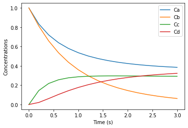
We next consider the two reactions A + B -> C and B + C -> D.
Here symbols A, B, C, D denote species concentrations in mol/L. The initial concentrations are \(A_0 = 1\), \(B_0 = 1\), \(C_0 = 0\), \(D_0 = 0\). We have \(k_1 = 1 \mathrm{L/mol \cdot s}\) and \(k_2 = 1.5\mathrm{L/mol \cdot s}\).
Reactions rates:
\[\begin{array}{l} \frac{dA}{dt} = -k_1 C_A C_B \\ \frac{dB}{dt} = -k_1 C_A C_B - k_2 C_B C_C \\ \frac{dC}{dt} = +k_1 C_A C_B - k_2 C_B C_C \\ \frac{dD}{dt} = + k_2 C_B C_C \end{array}\]# Simulate the reaction, with time step dt = 0.2s up to t=3s.
def rxn(Z, t):
k1 = 1
k2 = 1.5
r1 = k1*Z[0]*Z[1]
r2 = k2*Z[1]*Z[2]
dAdt = -r1
dBdt = -r1 - r2
dCdt = r1 - r2
dDdt = r2
# Return the derivatives.
return [dAdt, dBdt, dCdt, dDdt]
t = np.arange(0,3.01,0.2)
Z0 = [1,1,0,0]
# Integrate the ODE to get the concentrations
# Ca, Cb, Cc, Cd at each time t.
Conc = odeint(rxn, Z0, t)
# Plot the concentrations.
plt.plot(t, Conc[:,0])
plt.plot(t, Conc[:,1])
plt.plot(t, Conc[:,2])
plt.plot(t, Conc[:,3])
plt.xlabel('Time (s)')
plt.ylabel('Concentrations')
plt.legend(['Ca','Cb','Cc','Cd'])
plt.show()
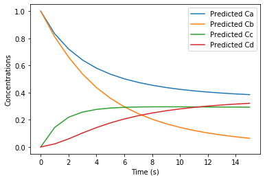
# Fitting a linear dynamical system to the time series data.
X = Conc.T
# Define a CVXPY variable for the dynamics matrix A.
A = cp.Variable((4,4))
# We predict the concentrations at time t+1 by multiplying
# the vector of concentrations at time t by the matrix A.
Xpred = A@X
# We find the A that minimizes the squared error
# of the prediction.
loss = cp.sum_squares(Xpred[:,:-1] - X[:,1:])
prob = cp.Problem(cp.Minimize(loss))
result = prob.solve()
print("The error in the linear dynamical system fit is", result)
print("The A matrix:")
print(A.value)

# Plot the predicted concentrations and the initial state.
Xplot = np.concatenate((X[:,:1], Xpred[:,:-1].value), axis=1)
plt.plot(Xplot.T)
plt.xlabel('Time (s)')
plt.ylabel('Concentrations')
plt.legend(['Predicted Ca','Predicted Cb','Predicted Cc','Predicted Cd'])
plt.show()
The error in the linear dynamical system fit is 5.35e-05
The A matrix:
[[ 0.45003437  0.38403464  0.17126201  0.41482706]
 [ 0.37614804  0.43544994  0.01111321 -0.37272932]
 [ 0.08661262  0.05684734  0.66858919  0.18708324]
 [ 0.07388633 -0.0514153   0.1601488   0.78755638]]
Again, if you found this note interesting or have any ideas, please reach out! (Contact info)